4. Running the First-Level Analysis

4.1. Specifying the Model

Having created the timing files in the previous chapter, we can use them in conjunction with our imaging data to create statistical parametric maps. These maps indicate the strength of the correlation between our ideal time-series (which consists of our onset times convolved with the HRF) and the time-series that we collected during the experiment. The amount of modulation of the HRF is represented by a beta weight, and this in turn is converted into a t-statistic when we create contrasts using the SPM contrast manager.

To begin, from the SPM GUI click on Specify 1st-Level. Note that the first field that needs to be filled in is the Directory field. Double-click on Directory and select the directory of the subject you want to analyse in 03_derivatives/spm-stats/first_level. All of the output of the 1st-level analysis will go into this folder.

Next, we will fill in the Timing parameters section. Under Units for design, select Seconds, and enter a value of 1.5 for Interscan Interval. Then click on Data & Design, and click five times on New: Subject/Session to create five new sessions. For the Scans of the first session, go to the func directory and use the Filter and Frames fields to select all 170 volumes of the warped and smoothed functional data (i.e., those files beginning with swu). Do the same for the volumes in the other sessions.

Go back to the field for the first session. Click on Multiple Conditions and then select the onset file correponding the that subject & run in 03_derivatives/spm-stats/onsets that you have previously created.

When you are done, save your batch in 03_derivatives/spm-stats/batches/ Then click the green Go button. The model estimation should only take a few moments. When it is finished, you should see something like this:

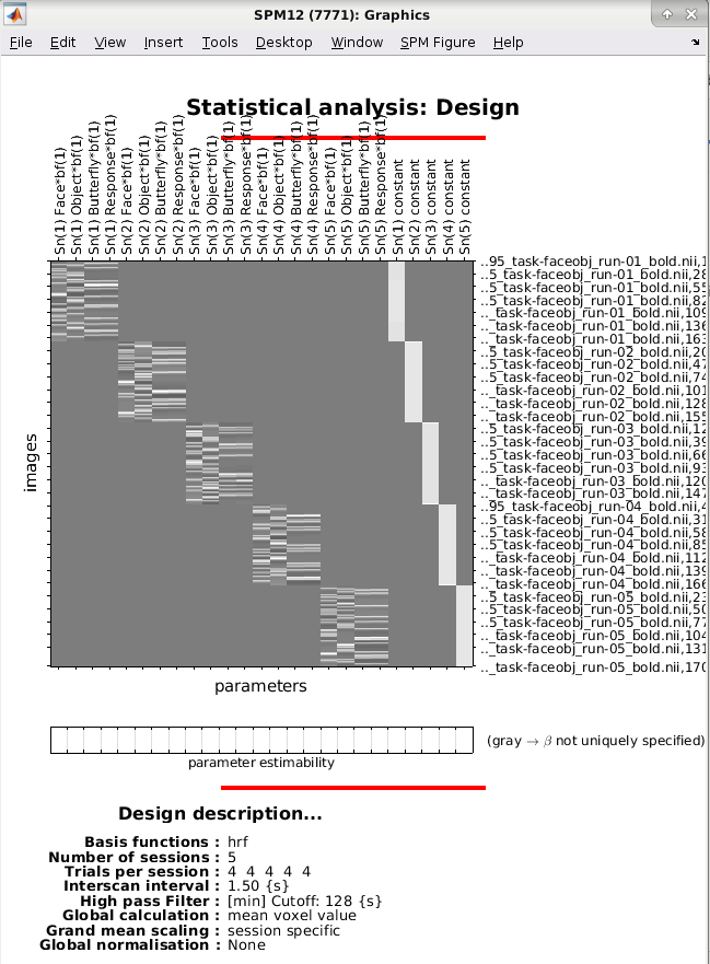
The General Linear Model for a single subject. The first four columns shows the time-series for the Face, Object, Butterfly and Motor Response conditions for the first session, while the next four show the ideal time-series for the conditions of run 2, ext. The last five columns are baseline regressors capturing the mean signal for each run. In this representation, time runs from top to bottom, and lighter colors represent more activity.

Important

Make sure the parameter estimability boxes are all white. If not there might be a problem with the onsets files

Exercise

In the bottom left SPM window, click on Design –> Design Orthogonality The labels on the right of the matrix are hard to read but they are the same as the top ones. This matrix represents the correlation between each regressor with the other. Two regressors are very correlated, can you spot them? Why are they so correlated? These two regressor will explain a substantial proportion of the same variance in the signal and cannot be both estimated accurately. In principle we should orthogonalize them before running the model estimation.

Now click on Design –> Explore and pick a Session and Condition. You should see something like this:

After pressing “Review”, selecting the pull-down ‘Design’ menu, Explore->Session, and selecting the regressor you wish to look at, you should get a plot similar to the one above. The top row shows time and frequency domain plots of the time-series corresponding to this regressor. In this particular case we have four events. Each event or “stick function” has been convolved with the hemodynamic response function shown in the bottom panel. The frequency domain graph is useful for checking that experimental variance is not removed by high-pass filtering. The grayed out section of the frequency plot shows those frequencies which are removed. For this regressor we have plenty of remaining experimental variance. Source: SPM12 manual

This figure shows the predicted signal time series in the top left graph, BOLD response shape in the bottom left and the signal that will be filtered out in the top right graph.

4.2. Estimating the Model

Now that we have created our GLM, we will need to estimate the beta weights for each condition. From the SPM GUI click Estimate, and then double-click on the field Select SPM.mat. Change the Write residuals option to No. Navigate to the first_Level directory and select the SPM.mat file, and then click the green Go button. This will take a few minutes to run.

4.3. The Contrast Manager

When you have finished estimating the model, you are ready to create contrasts. If we estimate a beta weight for the Faces condition and a beta weight for the Object condition, for example, we can take the difference between them to calculate a contrast estimate at each voxel in the brain. Doing so for each voxel will create a contrast map.

To create these contrasts, go back to the batch editor, select SPM -> Stats -> Contrast. Select the SPM.mat.

In the field Replicate over sessions, select Replicate. If you don’t choose Replicate, you will have to enter the 1 -1 0 0 sequence 5 times in the Weights vector box, in order to match the total number of regressors.

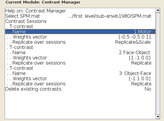
You can also create new contrast from the Results tool of the SPM GUI. After you select the SPM.mat file that was generated after estimating the model, you will see the design matrix on the right side of the panel. Click on Define New Contrast, and in the Name field type Face-Object. In the contrast vector window, type 1 -1 0 0 and repeat it 4 more time. Then click submit. If the contrast is valid, you should see green text at the bottom of the window saying “name defined, contrast defined”.

Make sure that you contrast manager looks like the figure below, and then click OK to create the contrast.

Note

If you forgot which column corresponds to which condition, hold down the right click button while hovering over one of the columns. You should see text that specifies which condition that column belongs to. You may have also noted that we used contrast weights of -0.5. Why those numbers, instead of the traditional 1 and -1? In this case, we are accounting for the unequal number of weights in the comparison. The sum of the weights should always be equal to 0.

Again, save your batch in 03_derivatives/spm-stats/batches/ and run the contrasts

4.4. Examining the Output

Click on Results button of the SPM GUI, select the SPM.mat and click on the contrast Face-Object to open the Results window. You will first need to set a few options:

1. apply masking: Set this to “none”, as we want to examine all of the voxels in the brain, and we do not want to restrict our analysis to a mask.

2. p value adjustment to control: Click on “none”, and set the uncorrected p-value to 0.001. This will test each voxel individually at a p-threshold of 0.001.

3. extent threshold {voxels}: Set this to 0 for now. This option will only show clusters of size bigger than the number of contiguous voxels you entered. It can be used to eliminate specks of voxels most likely found in noisy regions, such as the ventricles; later on we will learn how to do cluster correction at the group level to appropriately control for the number of individual statistical tests.

When you have finished specifying the options, you will see your results displayed on a glass brain. This shows your results in standardized space in three orthogonal planes, with the dark spots representing clusters of voxels that passed our statistical threshold. In the top-right corner is a copy of your design matrix and the contrast that you are currently looking at, and at the bottom is a table listing the coordinates and statistical significance of each cluster. The first column, set-level, indicates the probability of seeing the current number of clusters, c. The cluster-level column shows the significance for each cluster (measured in number of voxels, or kE) using different correction methods. The peak-level column shows the t- and z-statistics of the peak voxel within each cluster, with the main clusters marked in bold and any sub-clusters listed below the main cluster marked in lighter font. Lastly, the MNI coordinates of the peak for each cluster and sub-cluster is listed in the rightmost column.

If you left-click on the coordinates for a cluster, the coordinates will be highlighted in red and the cursor in the glass brain view will jump to those coordinates. You can click and drag the red arrow header in the glass brain if you like, and then right-click on the brain and select any of the options for jumping to the nearest suprathreshold voxel or the nearest local maximum.

To view the results on an image other than the glass brain, in the results window in the lower left (which contains the fields “p-values”, “Multivariate”, and “Display”), click on overlays and then select sections. Navigate to the spm12/canonical directory, and choose any of the T1 brains that you like.

You will now see the results displayed as a heatmap on the template, and you can click and drag the crosshairs as you do in the Display window. If you place the crosshairs over a particular cluster and click the “current cluster” button in the Results window, the statistical table will reappear, highlighting the coordinates of the cluster you have selected.

Note

If you want to quickly reload the display of the results on the template brain, click on overlays and select previous sections.

4.5. Exercises

1. Note the MNI coordinate of the peak voxel and identify the name of the brain region using an Atlas.

4.6. Next Steps

When you have finished running the preprocessing and first-level analyses, we will then need to run this for each subject in our study.

4.7. Video

For a video demonstration of how to do a 1st-level analysis in SPM, click here.