Looking at the Data
Now you will want to look at your data - for example, you will want to know if there are any artifacts or problems with your data, and whether these can be alleviated by preprocessing.
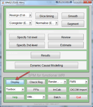
To look at and inspect the data, we will be using the SPM Graphical User Interface, or GUI for short. You can open the GUI by opening a new Matlab terminal, typing spm fmri from the command line, and pressing enter.
Inspecting the Anatomical Image
Whenever you download imaging data, check the anatomical and functional images for any artifacts - scanner spikes, incorrect orientation, poor contrast, and so on. It will take some time to develop an eye for what these problems look like, but with practice it will become quicker and easier to do.
To begin, let’s take a look at the anatomical image in the anat folder for sub-anwb1980.
If you haven’t already opened SPM, open matlab, select your working directory /home/lab1user/SHARED_labdata/PSYC724_LAB-DATA/02_rawdata/QA/ from the path bar at the top, or you can type in the matlab command window:
cd /home/lab1user/SHARED_labdata/PSYC724_LAB-DATA/02_rawdata/QA/
Then open the SPM graphical user interface. If you click on the Display button, you will be prompted to select an image. sub-anwb1980/anat/sub-anwb1980_T1w.nii
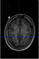
The anatomical image displayed in the SPM viewer in axial, sagittal, and coronal views. You can close any of the windows if you only want to focus on a subset of the views.
Inspect the image by clicking around in one of the viewing windows. Notice how the other viewing windows and crosshairs change as a result - this is because MRI data is collected as a three-dimensional image, and moving along one of the dimensions will change the other windows as well.
Now inspect your data in /home/lab1user/SHARED_labdata/PSYC724_LAB-DATA/02_rawdata for each participant.
Here are a few things to watch out for:
Lines that look like ripples in a pond. These are called Gibbs Ringing Artifacts, and they may indicate an error in the reconstruction of the MR signal from the scanner. These ripples may also be caused by the subject moving too much during the scan. In either case, if the ripples are large enough, they may cause preprocessing steps like brain extraction or normalization to fail.
The full brain should be present in the image and there should not be abnormal intensity differences within the grey or the white matter. The image quality should be good enough to identify the different structures of the brain and distinguish between tissue types.
The origin should be roughly in the center of the brain, near the posterior commissure (PC), and the image should be correctly oriented. If not, you may need to reset the origin (to the PC) and to reorient the image.
Make sure that the capsule appears on the left side. If it appear on the right, it may result from an issue during dicom –> nifti conversion.
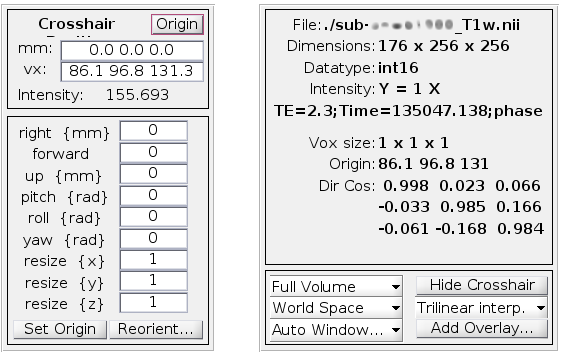
SPM displays some information about the volume, such as:
its dimension - the first number corresponds to the number of slices
the voxel size in mm
Inspecting the Functional Images
When you are done looking at the anatomical image, click on the Display button again, navigate to the func directory, and select the run-01 functional image.
Do the following exercice for the data in the QA folder first. Take notes of what excessive movements can do on image quality. Then look at the functional image for all your participants.
A new image will be displayed in the orthogonal viewing windows. This image also looks like a brain, but it is not as clearly defined as the anatomical image. This is because the resolution is lower. It is typical for a study to collect a high-resolution T1-weighted (i.e., anatomical) image and lower-resolution functional images, which are lower resolution in part because they are collected at a very fast rate. One of the trade-offs in imaging research is between spatial resolution and temporal resolution: Images collected at higher temporal resolution will have lower spatial resolution, and vice versa.

- Images can get lost when encoded or transferred between the scanner computer to the server. Very rare but can compromise the whole analysis. Make sure you have the expected number of volumes for your functional runs.
If you have fixed runs with a known duration, then the number of volumes = duration/TR
If your task is self-paced, or the acquisition had to be stopped manually, then - Record every trigger from the scanner in your task logfile, count them and make sure they correspond to the number of volumes. - Check that you have exactly 1 TR between the times of acquisition of every consecutive volumes.
Many of the quality checks for the functional image are the same as with the anatomical image: Watch out for extremely bright or extremely dark spots in the grey or white matter, as well as for image distortions such as abnormal stretching or warping. One place where it is common to see a little bit of distortion is in the orbitofrontal part of the brain, just above the eyeballs. There are ways to reduce this distortion, using the fieldmap that are located in the fmap folder, but we will not do it this time.
Another quality check is to make sure there isn’t excessive motion. Functional images are often collected as a time-series; that is, multiple volumes are concatenated together into a single dataset. To view the time-series of volumes in rapid succession, click the Check Reg button and load am image from one func folder. This will display a single volume in three planes: Coronal, Sagittal, and Axial. Right click on any of the planes and click the Browse button. You will be prompted to select an image; click on the currently selected file to remove it, and then enter the string run-01 in the Filter field, and 1:170 or Inf in the Frames field. Select all of the resulting images, and click Done.
You will now see a horizontal scrolling bar at the bottom of the display window. Clicking on the right or left arrows will advance or go back one volume; you can also click and drag the scrolling bar to view the volumes more rapidly. Clicking on the > button in the bottom right will start movie mode, which flips through the volumes at a rapid pace. Clicking on the button again will stop the movie. To see a plot of the time-series activation at the voxel under the crosshairs, right-click again on any of the planes, select “Browse”, and then select “Display profile”. This opens up another figure that you can view simultaneously as you flip through the volumes.

Also, during the Realignment preprocessing step, you will generate a movement parameter file showing how much motion there was between each volume.
Exercises
View the time-series of the data from all the runs form a given subject, using the steps outlined above. Do you notice any sudden changes in movement?
Note
Each student should select a different subject, so that all the data is viewed.
Examine a few of the other anatomical and functional scans for some of the other subjects. How does the contrast and the brightness change as you drag the crosshair through different slices of the image? What do you think affects the brightness of a given slice?
Open the anatomical image for your subject in the Display Image viewer, and right click on any of the three window panes. Select
Overlay -> Add Image -> This Image, and select the first functional file. The functional image will be overlaid on the anatomical image and displayed in a red-orange heatmap, the initial alignment between the images:
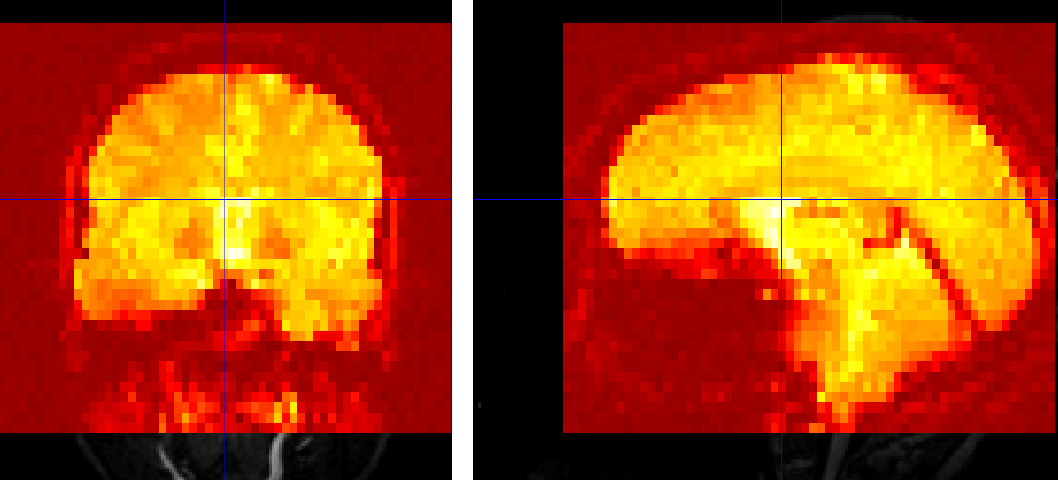
Here is an exemple of a bad alignment:

What do you notice? If you find some misalignement, you should address it by following instructions for the chapter on Setting the origin.
Video
For a video overview of how to check the quality of your data, click here.